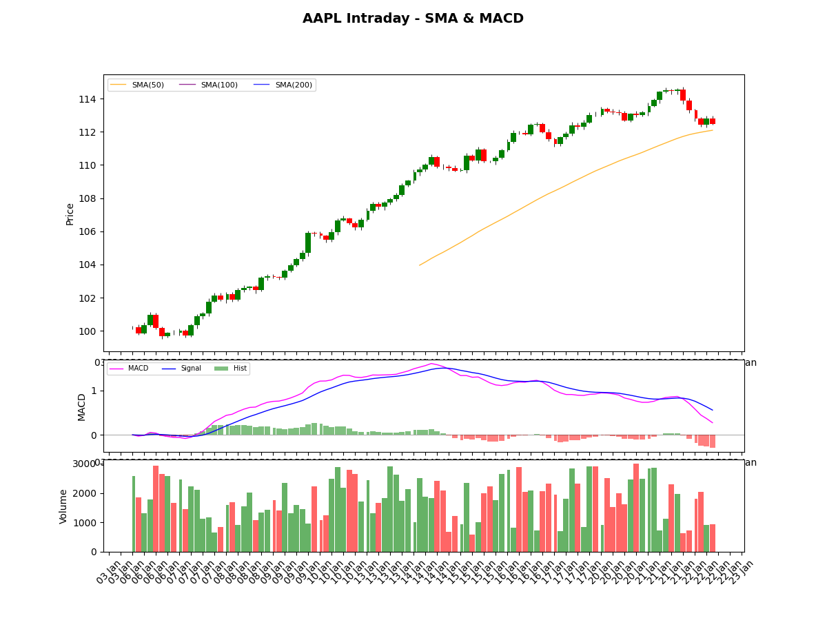
Multi-Panel Financial Chart¶

AAPL Intraday - SMA & MACD

Out:

/Users/simonniederberger/Library/CloudStorage/Dropbox/Git/busdayaxis/examples/financial_plots/plot_stock_macd.py:124: UserWarning: This figure includes Axes that are not compatible with tight_layout, so results might be incorrect.
  _ = plt.tight_layout(rect=[0, 0, 1, 0.96])

import matplotlib.dates as mdates
import matplotlib.pyplot as plt
import numpy as np
import pandas as pd

import busdayaxis

busdayaxis.register_scale()

rng = np.random.default_rng(42)
n = 100

# Generate ~30 days of hourly data (excluding weekends)
hours = list(range(9, 17))  # 9am-4pm
start_date = pd.Timestamp("2025-01-06")

# Create business days and hours
all_times = []
current = start_date
while len(all_times) < n:
    if current.weekday() < 5:  # Mon-Fri
        for h in hours:
            all_times.append(current + pd.Timedelta(hours=h))
    current += pd.Timedelta(days=1)

bar_idx = pd.DatetimeIndex(all_times[:n])

# Generate price data with trend
returns = rng.normal(0.0005, 0.005, n)
trend = np.linspace(0, 0.1, n)  # slight upward trend
close = 100 * (1 + trend + pd.Series(returns).cumsum()).values

# Create OHLC
open_ = np.roll(close, 1)
open_[0] = close[0]
high = np.maximum(open_, close) + rng.uniform(0.05, 0.2, n)
low = np.minimum(open_, close) - rng.uniform(0.05, 0.2, n)

# Colors
colors = ["green" if c >= o else "red" for c, o in zip(close, open_)]
body_bottom = np.minimum(open_, close)
body_height = np.abs(close - open_)

# Volume
volume = rng.integers(500, 3000, n)

# Moving Averages
sma50 = pd.Series(close).rolling(50).mean().values
sma100 = pd.Series(close).rolling(100).mean().values
sma200 = pd.Series(close).rolling(200).mean().values

# MACD (12, 26, 9)
ema12 = pd.Series(close).ewm(span=12, adjust=False).mean()
ema26 = pd.Series(close).ewm(span=26, adjust=False).mean()
macd_line = ema12 - ema26
signal_line = macd_line.ewm(span=9, adjust=False).mean()
macd_hist = macd_line - signal_line

# Layout: 3 panels
fig = plt.figure(figsize=(12, 9))
gs = fig.add_gridspec(3, 1, height_ratios=[3, 1, 1], hspace=0.05)

ax_price = fig.add_subplot(gs[0])
ax_macd = fig.add_subplot(gs[1], sharex=ax_price)
ax_vol = fig.add_subplot(gs[2], sharex=ax_price)

fig.suptitle("AAPL Intraday - SMA & MACD", fontsize=14)

bar_width = pd.Timedelta(minutes=55)

# --- Price Panel ---
# Wicks
ax_price.vlines(bar_idx, low, high, linewidth=0.6, color="black", zorder=3)
# Bodies
ax_price.bar(
    bar_idx,
    body_height,
    bottom=body_bottom,
    width=bar_width,
    color=colors,
    zorder=4,
)
# Moving Averages
ax_price.plot(bar_idx, sma50, color="orange", linewidth=1, label="SMA(50)", alpha=0.8)
ax_price.plot(bar_idx, sma100, color="purple", linewidth=1, label="SMA(100)", alpha=0.8)
ax_price.plot(bar_idx, sma200, color="blue", linewidth=1, label="SMA(200)", alpha=0.8)

ax_price.set_ylabel("Price")
ax_price.legend(loc="upper left", fontsize=8, ncol=3)
ax_price.tick_params(axis="x", labelbottom=False)

# --- MACD Panel ---
ax_macd.plot(bar_idx, macd_line.values, color="fuchsia", linewidth=1, label="MACD")
ax_macd.plot(bar_idx, signal_line.values, color="blue", linewidth=1, label="Signal")
# Histogram as bars
hist_colors = ["green" if h >= 0 else "red" for h in macd_hist.values]
ax_macd.bar(
    bar_idx,
    macd_hist.values,
    width=bar_width,
    color=hist_colors,
    alpha=0.5,
    label="Hist",
)
ax_macd.axhline(0, color="black", linewidth=0.5, alpha=0.5)
ax_macd.set_ylabel("MACD")
ax_macd.legend(loc="upper left", fontsize=7, ncol=3)
ax_macd.tick_params(axis="x", labelbottom=False)

# --- Volume Panel ---
ax_vol.bar(bar_idx, volume, color=colors, alpha=0.6, width=bar_width)
ax_vol.set_ylabel("Volume")

ax_vol.xaxis.set_major_locator(busdayaxis.DayLocator())
ax_vol.xaxis.set_major_formatter(mdates.DateFormatter("%d"))

# --- Apply busday scale ---
for ax in [ax_price, ax_macd, ax_vol]:
    ax.set_xscale("busday", bushours=(9, 17))

_ = plt.tight_layout(rect=[0, 0, 1, 0.96])

Total running time of the script: ( 0 minutes 1.149 seconds)

Download Python source code: plot_stock_macd.py

Download Jupyter notebook: plot_stock_macd.ipynb

Gallery generated by mkdocs-gallery