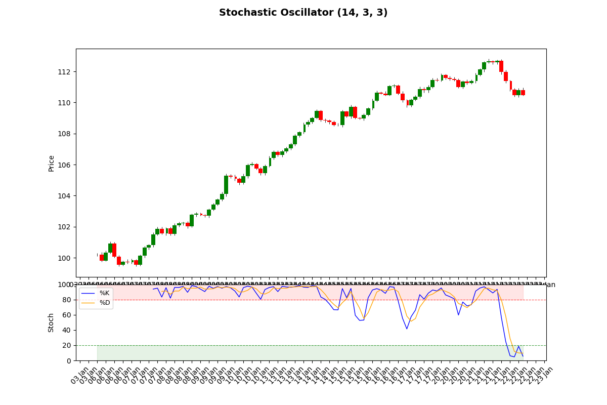
Chart with Stochastic Oscillator¶

Stochastic Oscillator (14, 3, 3)

Out:

/Users/simonniederberger/Library/CloudStorage/Dropbox/Git/busdayaxis/examples/financial_plots/plot_stock_stochastic.py:87: UserWarning: This figure includes Axes that are not compatible with tight_layout, so results might be incorrect.
  _ = plt.tight_layout(rect=[0, 0, 1, 0.96])

import matplotlib.dates as mdates
import matplotlib.pyplot as plt
import numpy as np
import pandas as pd

import busdayaxis

busdayaxis.register_scale()

rng = np.random.default_rng(42)
n = 100
# Generate hourly data
hours = list(range(9, 17))
all_times = []
current = pd.Timestamp("2025-01-06")
while len(all_times) < n:
    if current.weekday() < 5:
        for h in hours:
            all_times.append(current + pd.Timedelta(hours=h))
    current += pd.Timedelta(days=1)

bar_idx = pd.DatetimeIndex(all_times[:n])
n = len(bar_idx)

# Price data
returns = rng.normal(0.0005, 0.005, n)
trend = np.linspace(0, 0.08, n)
close = 100 * (1 + trend + pd.Series(returns).cumsum()).values

# OHLC
open_ = np.roll(close, 1)
open_[0] = close[0]
high = np.maximum(open_, close) + rng.uniform(0.05, 0.15, n)
low = np.minimum(open_, close) - rng.uniform(0.05, 0.15, n)

colors = ["green" if c >= o else "red" for c, o in zip(close, open_)]
body_bottom = np.minimum(open_, close)
body_height = np.abs(close - open_)

# Stochastic Oscillator (14, 3, 3)
lowest_low = pd.Series(low).rolling(14).min()
highest_high = pd.Series(high).rolling(14).max()
stoch_k = 100 * (close - lowest_low) / (highest_high - lowest_low)
stoch_d = stoch_k.rolling(3).mean()

# Layout
fig = plt.figure(figsize=(12, 8))
gs = fig.add_gridspec(2, 1, height_ratios=[3, 1], hspace=0.05)

ax_price = fig.add_subplot(gs[0])
ax_stoch = fig.add_subplot(gs[1], sharex=ax_price)

fig.suptitle("Stochastic Oscillator (14, 3, 3)", fontsize=14)

bar_width = pd.Timedelta(minutes=55)

# --- Price Panel ---
ax_price.vlines(bar_idx, low, high, linewidth=0.6, color="black", zorder=3)
ax_price.bar(
    bar_idx, body_height, bottom=body_bottom, width=bar_width, color=colors, zorder=4
)
ax_price.set_ylabel("Price")

# --- Stochastic Panel ---
ax_stoch.plot(bar_idx, stoch_k.values, color="blue", linewidth=1, label="%K")
ax_stoch.plot(bar_idx, stoch_d.values, color="orange", linewidth=1, label="%D")
ax_stoch.axhline(80, color="red", linestyle="--", linewidth=0.8, alpha=0.7)
ax_stoch.axhline(20, color="green", linestyle="--", linewidth=0.8, alpha=0.7)

# Shade zones
ax_stoch.fill_between(bar_idx, 80, 100, alpha=0.1, color="red")
ax_stoch.fill_between(bar_idx, 0, 20, alpha=0.1, color="green")

ax_stoch.set_ylabel("Stoch")
ax_stoch.set_ylim(0, 100)
ax_stoch.legend(loc="upper left", fontsize=9)

ax_price.tick_params(axis="x", labelbottom=False)
ax_stoch.xaxis.set_major_locator(busdayaxis.DayLocator())
ax_stoch.xaxis.set_major_formatter(mdates.DateFormatter("%d %b"))
ax_price.set_xscale("busday", bushours=(9, 17))
ax_stoch.set_xscale("busday", bushours=(9, 17))

_ = plt.tight_layout(rect=[0, 0, 1, 0.96])

Total running time of the script: ( 0 minutes 0.282 seconds)

Download Python source code: plot_stock_stochastic.py

Download Jupyter notebook: plot_stock_stochastic.ipynb

Gallery generated by mkdocs-gallery